A while ago I came up with an idea for a website which shows the current liturgical colour of the Church of England. The website has the catchy name of Liturgical Colour and is now publicly available at https://liturgical.uk/
I also added an API which allows anyone to query the data progammatically. This is available at https://api.liturgical.uk/today and returns output like:
Still not satisfied, I decided to work on a smart table lamp that would be able to show the current liturgical colour. I have no experience in electronics or embedded computing, so I decided to use off-the-shelf smart lights and Home Assistant (not that I’ve got any experience with those either).
At the time I made the purchase, the cheapest RGB smart light that claimed to be compatible with Home Assistant. It happened to be a Wiz model, but the brand shouldn’t matter, so long as it work with Home Assistant. These instructions should be sufficiently generic.
Home Assistant setup
This guide assumes you have already installed a basic instance of Home Assistant.
It also assumes you have followed the smart light manufacturer’s instructions to get the light set up in Home Assistant.
Liturgical API Integration
First we need to configure this as an Integration in Home Assistant, using the RESTful integration. Unfortunately this can only be configured using the config file configuration.yaml and not via the UI.
Copy this config chunk into your configuration.yaml verbatim. It will poll the Liturgical API hourly and various various pieces of information as “sensors”.
Restart your Home Assistant instance. You should now be able to see a section called Sensors with various pieces of information, which we will be able to use in some automation.
Automations
Now we need to create some Automations to take the output from the Liturgical API and use the information to set the colour on the lamp.
In theory, an RGBW lamp should be able to display pure white, but on the lamp I tested, setting RGBW mode to pure white actually yielded a weird peach colour. As a workaround, we will create one automation for all the “colour” days and a separate automation for the “white” days which uses colour temperature mode instead, to achieve a proper white.
Setting up Automations via the UI is a bit fiddly and requires a lot of clicking, so again we will define them in configuration.yaml. Add the following section to create your automations. Be sure to change references to light.wiz_rgbw_tunable_04370c to your own lamp. You can check this ID by browsing Entities in the UI.
automation liturgical:
  - alias: Liturgical colour on (colour days)
    description: Switch on lamp at sunrise in RGBW mode, if it is a non-white colour day
    triggers:
      - trigger: sun
        event: sunrise
        offset: 0
    conditions:
      - or:
          - condition: state
            entity_id: sensor.liturgical_colour
            state:
              - purple
          - condition: state
            entity_id: sensor.liturgical_colour
            state:
              - red
          - condition: state
            entity_id: sensor.liturgical_colour
            state:
              - green
          - condition: state
            entity_id: sensor.liturgical_colour
            state:
              - rose
    actions:
      - target:
          entity_id: light.wiz_rgbw_tunable_04370c
        action: light.turn_on
        data:
          rgbw_color: "{{ states('sensor.liturgical_colour_code_rgbw') }}"
    mode: single

  - alias: Liturgical colour on (white)
    description: Switch on lamp at sunrise in colour temperature mode, if it is a white day
    triggers:
      - trigger: sun
        event: sunrise
        offset: 0
    conditions:
      - condition: state
        entity_id: sensor.liturgical_colour
        state:
          - white
    actions:
      - action: light.turn_on
        metadata: {}
        data:
          color_temp_kelvin: 6000
        target:
          entity_id: light.wiz_rgbw_tunable_04370c
    mode: single

  - alias: Liturgical off
    description: Switch off lamp at 11pm
    triggers:
      - trigger: time
        at: "23:00:00"
        weekday:
          - mon
          - tue
          - wed
          - thu
          - fri
          - sat
          - sun
    conditions: []
    actions:
      - action: light.turn_off
        metadata: {}
        data: {}
        target:
          entity_id: light.wiz_rgbw_tunable_04370c
    mode: single
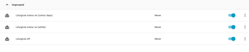
The Automations UI should look similar to this, and you should now have a smart light that illuminates in daylight hours, showing the current liturgical colour.
On my Kubernetes homelab, I am running a handful of workloads that support GPU hardware acceleration, so I decided to look into it.
I had to do a lot of reading different sources to figure out how to put this together, and so I present my findings here so hopefully someone else can benefit. Many of the existing documents also recommend installing components by simply applying kube manifests from GitHub to their cluster. I don’t like doing this, so wherever possible I will use Helm charts to do managed installations.
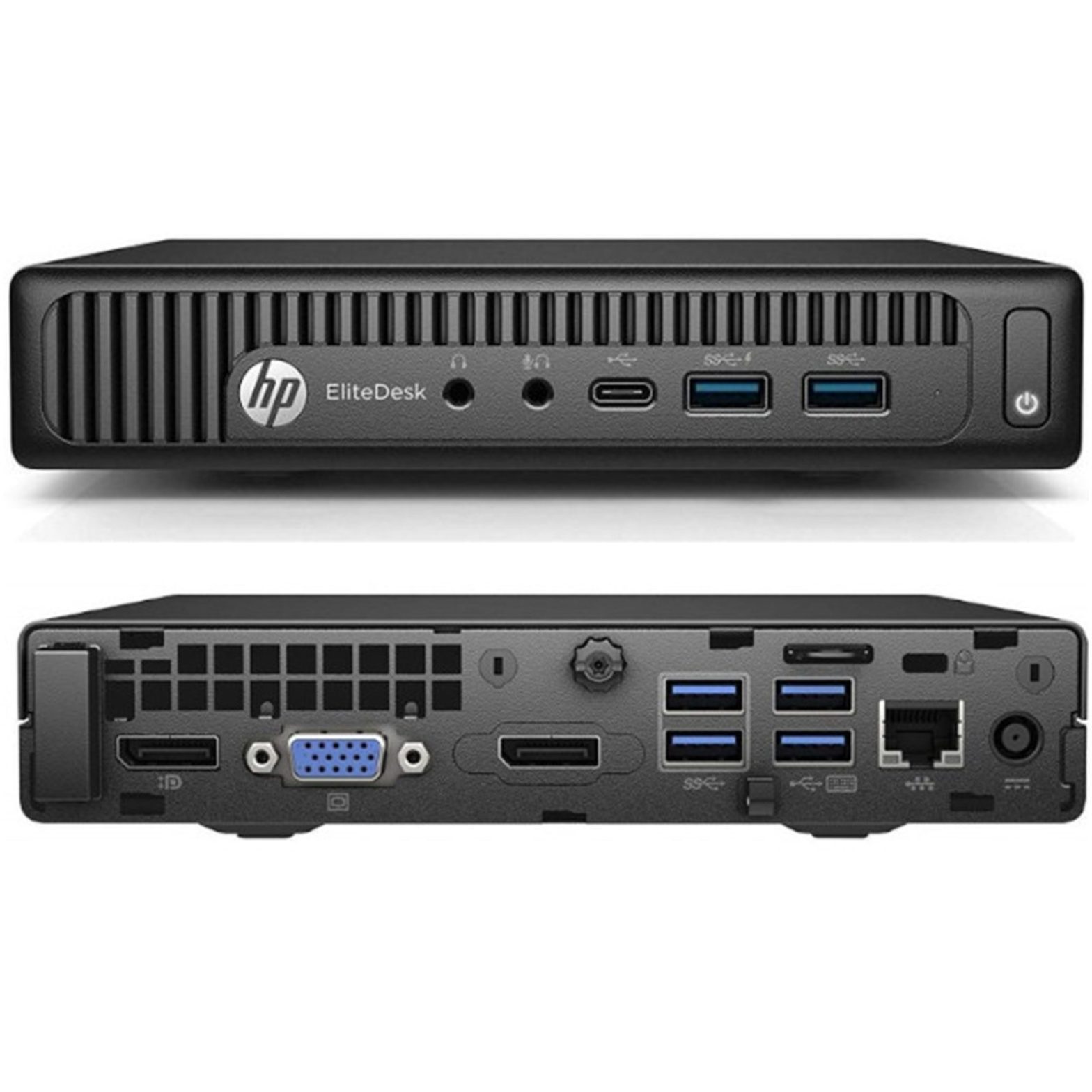
My hardware consists of HP EliteDesk 800 G2 mini PCs, which have an Intel i5-6500T CPU and the integrated Intel HD Graphics 530. This onboard chip is hardly going to offer mind-blowing performance, but it’s better to use it than for it to sit idle! And it may even offer reasonable performance for some tasks, while freeing up the CPU.
People who are serious about their GPU acceleration will presumably have discrete GPUs, most likely from NVIDIA or AMD. This guide will focus specifically on Intel GPUs, because that is what I have, and because the documentation around an end-to-end Intel GPU acceleration in Kubernetes seems lacking.
node-feature-discovery
The first component we need is Node Feature Discovery (NFD). This is an add-on published by a Kubernetes SIG which collects details about the hardware available on each node, and exposes that information as node labels. NFD is a framework, and allows adding custom rules to discover and advertise arbitrary features.
Now we need to supply node-feature-discovery with some extra detection rules so it can recognise Intel hardware. Unfortunately this is just a manifest that has to be applied.
Check that the nodes with GPUs are now labelled. There will be a set of new feature.node.kubernetes.io labels, but the additional detection rules we added should also create some intel.feature.node.kubernetes.io and gpu.intel.com labels – provided your system has an Intel GPU.
P.S. the autonodelabel.io labels come from my own project.
intel-device-plugin
Now we need to install the Intel device plugin. This is a two-part operation. First we need to install Intel’s device plugins operator. Default values are fine.
Once the operator has fired up, we can use it to install Intel’s GPU plugin. This time we do need to provide a minimal values file to tell the plugin to run only on nodes which have an Intel GPU (based on the labels added by node-feature-discovery in the previous step):
When the driver is initialised, we can see that the nodes with compatible GPUs now have GPU as a requestable resource, along with the CPU and memory. Note this isn’t a generic gpu key, but specific to the Intel i915 driver. You would see something different here if you were using NVIDIA or AMD GPUs.
Once Kubernetes is aware of the GPU hardware and able to expose it to pods, we need to verify which codecs and APIs are available. This is all new to me so I had a lot of learning to do, but each specific hardware platform needs a suitable driver, and the driver interfaces with an API which is presented to workloads.
In my particular case, running the vainfo command on the nodes reveals that I’m running the Intel iHD driver, which supports both Intel QSV and VA-API as APIs to present to the application.
Finally, we can starting deploying workloads that can use these APIs to request GPU acceleration for some tasks. These examples are just arbitrary apps that I happen to be using at home.
Jellyfin
Jellyfin is an open source media server, similar to Plex. It can use a GPU to perform realtime transcoding when streaming video.
I deploy Jellyfin using a Helm chart of my own creation. This minimal values.yaml shows the bare minimum config to set to enable hardware transcoding.
---
# Jellyfin requests 1 GPU so it gets scheduled on a compatible node
resources:
  jellyfin:
    requests:
      cpu: 1000m
      memory: 1Gi
      gpu.intel.com/i915: "1"
    limits:
      cpu: 3500m
      memory: 6Gi
      gpu.intel.com/i915: "1"

# Generous permissions to allow Jellyfin to access GPU hardware
podSecurityContext:
  runAsNonRoot: false
  fsGroup: 64710
  seccompProfile:
    type: RuntimeDefault
  runAsUser: 64710
  runAsGroup: 64710
  supplementalGroups:
    - 109
containerSecurityContext:
  privileged: true
  allowPrivilegeEscalation: true
  capabilities:
    drop:
      - ALL
  readOnlyRootFilesystem: true
  runAsNonRoot: false
  runAsUser: 64710
  runAsGroup: 64710

# Tell Jellyfin to mount the GPU device from the host
jellyfin:
  extraDevices:
    - /dev/dri/renderD128
Finally, with the Jellyfin deployment made, we need to go into the administration settings in the web console and enable hardware acceleration. These onboard Intel GPUs support both QSV and VA-API so either should work. There is a lot of debate about performance vs quality online, but I’ve been using QSV and it has been fine on this modest hardware. If you have only one GPU, there is no need to set the QSV device.
Configuring transcoding on Jellyfin
It is a bit difficult to verify that your Jellyfin hardware acceleration is working. The Jellyfin pod logs are messy, but look for a line that mentions Transcoding when starting to play a video. See that it mentions -codec:v:0 h264_qsv which means the video codec to transcode to is h264_qsv, so it is using QSV on the GPU to perform this transcode.
Be aware that not every playback results in a video being transcoded! If your client supports the codec that the video is already in, it won’t transcode. Check the transcoding docs for more details.
Immich is a self-hosted photo gallery app. It can make use of a GPU in a couple of ways.
Hardware transcoding
Firstly, Immich can use a GPU to transcode video clips in your library, much the same as Jellyfin can.
I am deploying Immich from their own Helm chart. It’s a fairly complex deployment, but the relevant section of values.yaml to enable hardware transcoding is this section below. This just tells Kubernetes to schedule the Immich server on a node with a GPU.
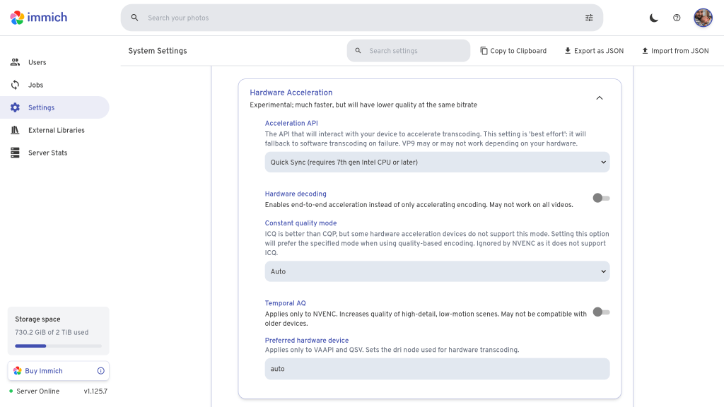
As with Jellyfin, we need to actually configure hardware acceleration in the Immich GUI. Click your user avatar, go to Administration, Settings, scroll down to Video Transcoding Settings, and go to Hardware Acceleration. Once again, we have the choice of QSV or VA-API, and I have chosen QSV.
Immich Hardware Acceleration settings for Transcoding
Correct behaviour is a bit harder to verify in Immich. I uploaded some videos to my library but wasn’t able to trigger any transcoding. Maybe it only does that for longer videos – I’m not sure.
The more interesting use of GPU acceleration in Immich is machine learning, which it uses for facial recognition and auto tagging images based on their content. The ML component of Immich runs as a separate pod with its own config. This means if you are running a single node cluster, you will need to share the GPU between the server pod and the ML pod, by setting requests to 500m each.
The relevant part of the values.yaml to share is below. Here we have to make three changes.
Firstly we have to run an alternative version of the ML image with support for OpenVINO, which is the ML framework for Intel GPUs (the default ML image targets NVIDIA hardware).
Secondly, we specify the Intel GPU in the resources section as usual
Thirdly, and optionally, we set a couple of environment variables to tell the pod to preload the ML models at container startup and set some more generous startup probes, as it takes a little bit of time to preload. If you don’t do this step, the pod will load the ML models the first time it needs them.
machine-learning:
  enabled: true
  image:
    # Specify OpenVINO image variant for Intel
    tag: main-openvino
  env:
    # Load ML models up front
    MACHINE_LEARNING_PRELOAD__CLIP: ViT-B-32__openai
    MACHINE_LEARNING_PRELOAD__FACIAL_RECOGNITION: buffalo_l
  resources:
    requests:
      memory: 4Gi
      cpu: 750m
      gpu.intel.com/i915: 1
    limits:
      gpu.intel.com/i915: 1
  # Override probes to allow slow ML startup
  probes:
    liveness:
      spec:
        initialDelaySeconds: 120
    readiness:
      spec:
        initialDelaySeconds: 120
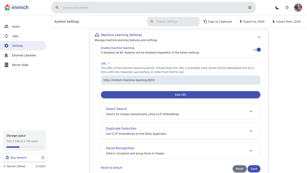
There are fewer settings for ML hardware acceleration. In fact, all we need to do is enable ML in Immich settings and it will automatically pick up any available GPU.
ML settings in Immich
Verification of correct hardware acceleration config for ML is easy to spot. When the ML pod starts up, it prints an message like this. If the message has OpenVINOExecutionProvider first, it’s working. If you only have CPUExecutionProvider, it hasn’t worked.
[02/11/25 19:12:36] INFO Setting execution providers to ['OpenVINOExecutionProvider','CPUExecutionProvider'], in descending order of preference
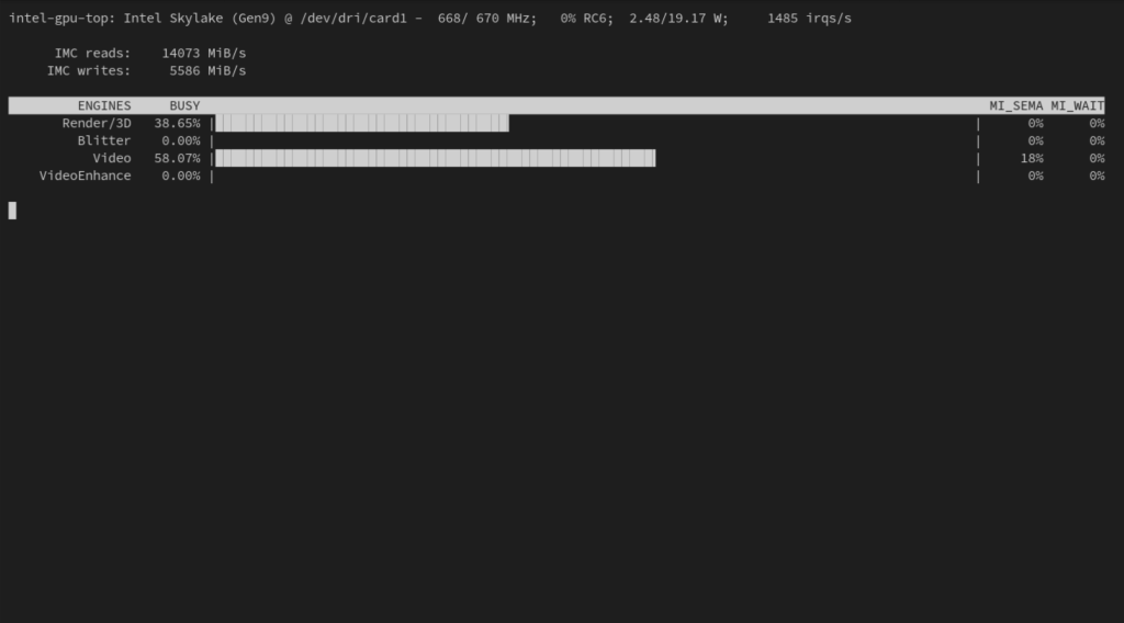
There is a tool called intel_gpu_top which works the same spirit as Linux’s top command. It shows what the GPU is up to and which of the filters are being used, so it’s handy for observing the node that your workloads are on, to make sure they are using hardware acceleration.
It can be installed on the Kubernetes node (not in the cluster) with:
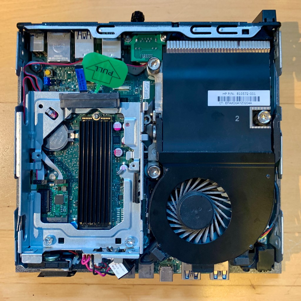
I use a stack of HP EliteDesk G2 Minis to run a Kubernetes cluster at home. While they are several years old now, they’re still useful because of their low power consumption. Plus, I’m a cheapskate and I hate spending money, so I bought old PCs and I’ve upgraded them in every way I can. I’ve maxed out the memory to 32GB and added an NVMe SSD to provide clustered storage with Ceph.
It’s actually Ceph that led me to discover a bottleneck. These little systems only have 1GbE on board, and when you have clustered storage, suddenly the nodes need to do a lot of I/O to each other. They easily saturate a 1Gbit network link while syncing a Ceph storage device.
So I looked for the best cheapest way to add 2.5Gbit network support to these tiny computers. I didn’t want USB dongles hanging out the back, so I looked for internal options.
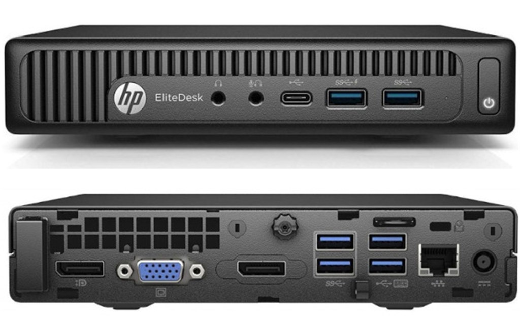
I noticed the G2 Mini has some kind of modular option on the back – in the photo above, it has a second DisplayPort port. Turns out you can get various proprietary daughterboards to fit in these with different ports on, but none have 2.5GbE in this generation.
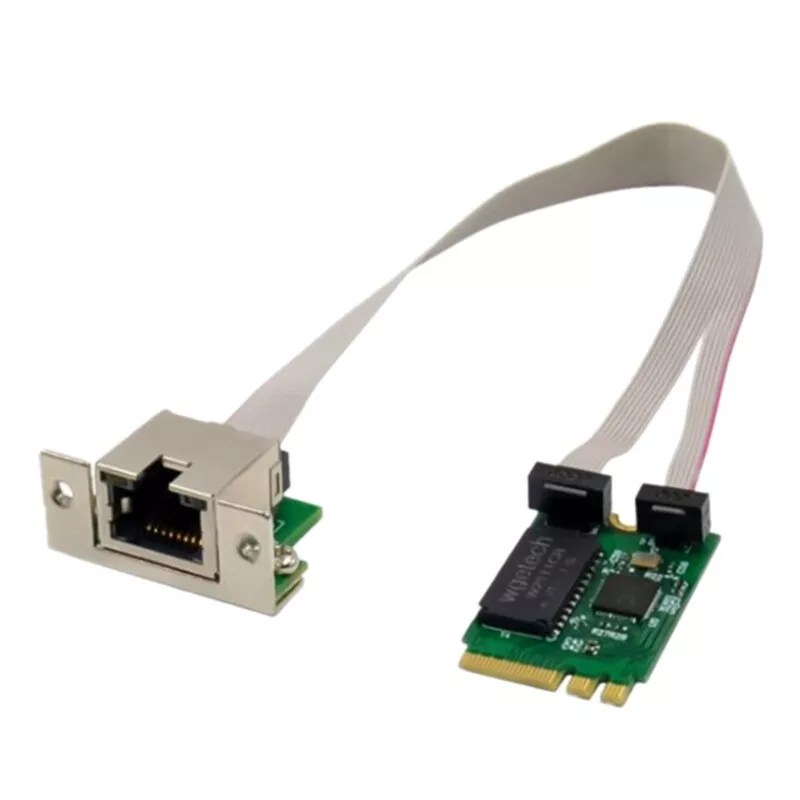
As well as the M.2 NVMe slot for storage, the G2 Mini also has an M.2 Key A+E slot, which is typically populated with the Wi-Fi/Bluetooth card. As I’m not using Wi-Fi in mine, I searched for M.2 A+E 2.5GbE network adapters, and was pleased to find plenty of cheap no-name adapters on eBay. There isn’t much information available in the eBay listings, but it looked like they “might” fit, so I ordered one to have a closer look.
M.2 A+E 2.5GbE network adapter
While these adapters don’t have a prominent brand name on them, the chipset is a Realtek RTL8125, which is a well known brand and has support in various operating systems.
Different variants of this device are available, but you need to order one that has the following characteristics, otherwise it won’t physically fit:
Key A+E interface (two notches in the contacts on the same side)
A single, central retaining screw at the opposite edge of the card
A cable with a split to go around the retaining screw, and two push-on connectors
Connectors which come out at 90° – sideways, not upwards
Fitting one of these network adapters into the G2 Mini is a fiddly process and requires a few modifications. I’ve now modded all 6 of my Kubernetes nodes with this procedure, and I have documented the procedure with photos, in the unlikely event that someone else also wants to add 2.5GbE to their old G2 Minis.
You will need
HP EliteDesk G2 Mini or similar
Generic M.2 A+E 2.5GbE network card
Small Phillips or Pozi screwdriver
Flat blade screwdriver
Junior hacksaw
Pliers
Metal file
M3x8mm bolts, qty 2
M3 washers, qty 2
Thermal paste
Alcohol wipes
How to do it
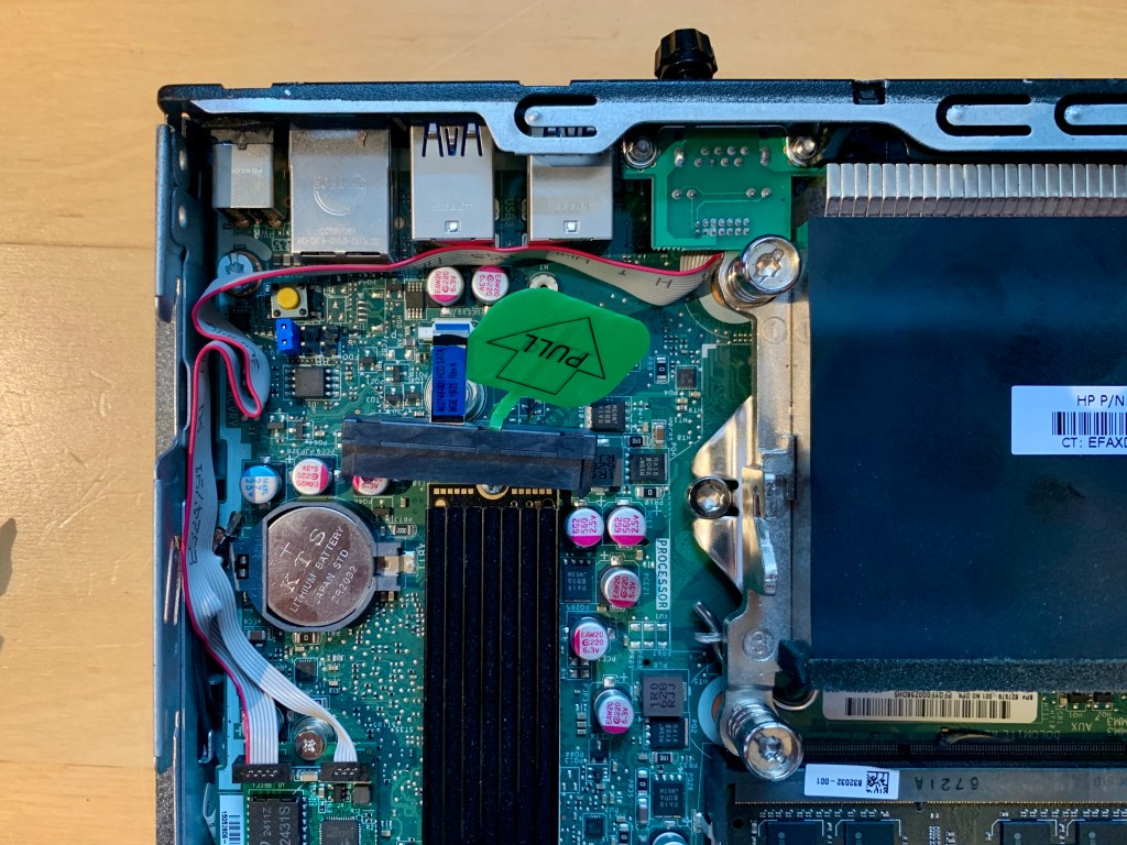
Take the lid off the G2 Mini. Gently pull out the SATA connector from the 2.5″ SSD, if fitted, then remove the SSD from its cage by pulling the metal latch sideways and sliding the SSD towards the rear of the machine before lifting it out.
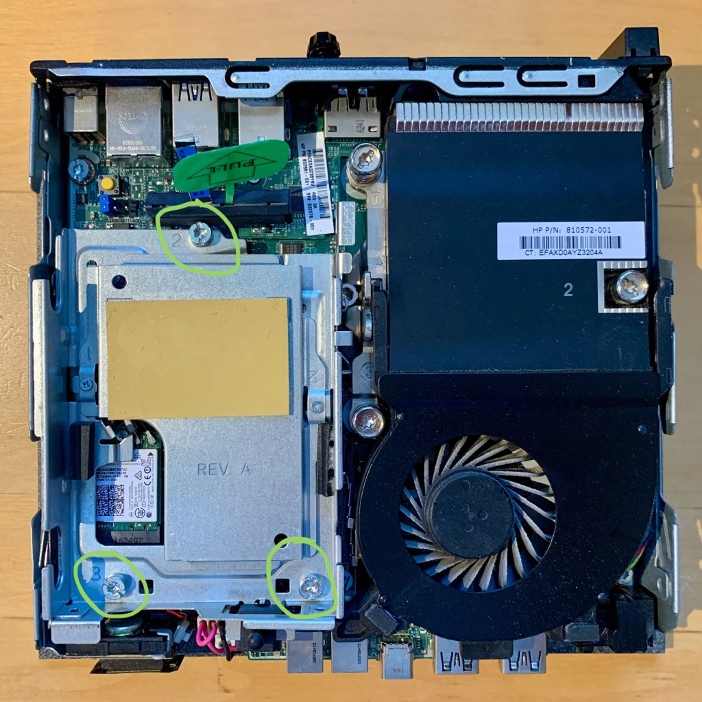
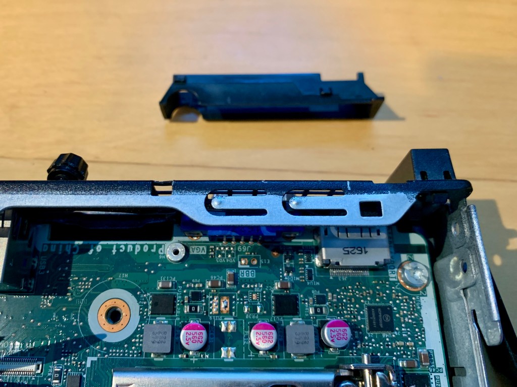
HP G2 Mini showing location of drive cage boltsRemove the lid sensor
Undo the three bolts which hold the drive cage in place. Make sure to slide the case open sensor out of the drive cage. Put the cage to one side.
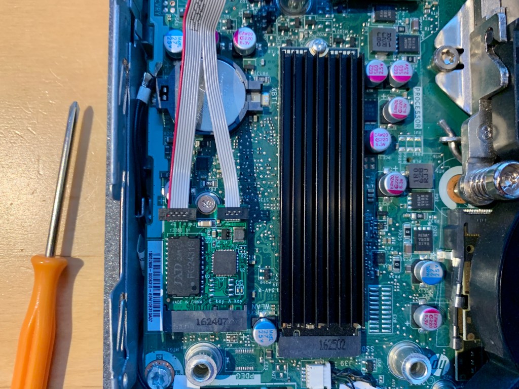
Location of Wi-Fi card
If your system has a Wi-Fi card fitted, carefully remove the two antenna cables by lifting the gold connectors away from the board with a table knife (or similar). Tuck the antenna wires down the side of the motherboard to keep them out of the way. Undo the retaining screw to remove the card.
Replacement 2.5GbE card
Fit the 2.5GbE card in its place and replace the retaining screw.
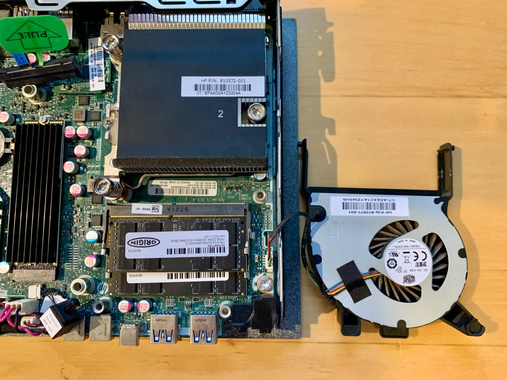
Remove the fan
Remove the system fan by gently lifting up the black plastic tab to rotate the fan unit upwards, then sliding towards the front of the machine to free it. Place it to one side, being careful not to pull the cable.
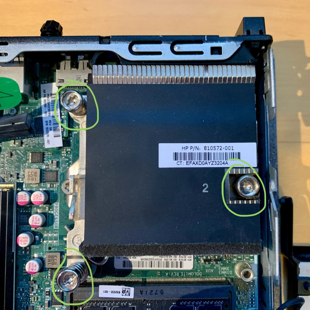
Location of CPU heat sink screws
Remove the three CPU heat sink screws. You can use either a Torx or a flat head screwdriver. Flip the heat sink over, and place it to one side. Try not to get thermal paste on anything! Clean the CPU and heat sink with alcohol wipes.
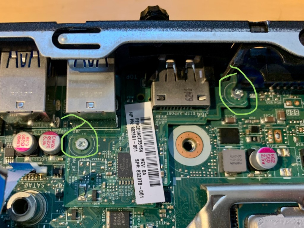
Location of daughterboard screws
With the heat ink out of the way, undo the two small screws that hold the daughterboard in place. Use a knife or flat screwdriver to lift the daughterboard up from the motherboard. Remove the daughterboard – sometimes it gets stuck to the foam around the opening in the case.
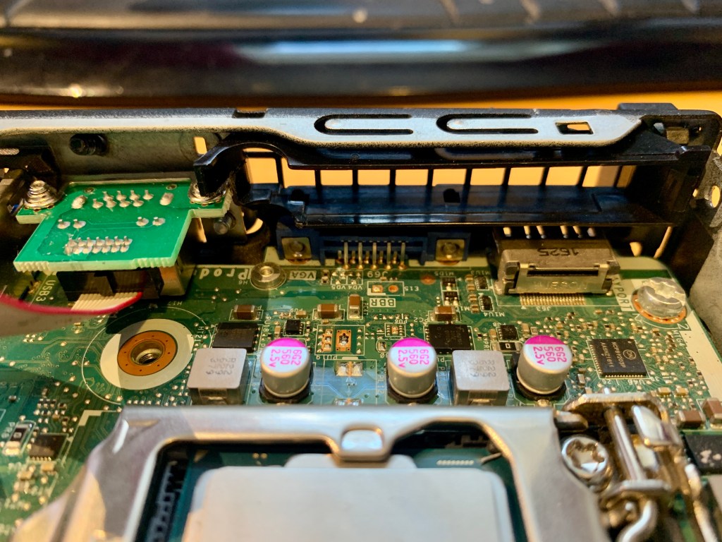
Heat sink shroud
Unclip and remove the black plastic shroud from behind the heat sink.
The hatched area needs to be removed
Use a junior hacksaw to remove the area of plastic that I have hatched in the above picture. This is to allow clearance for the corner of the RJ45 port.
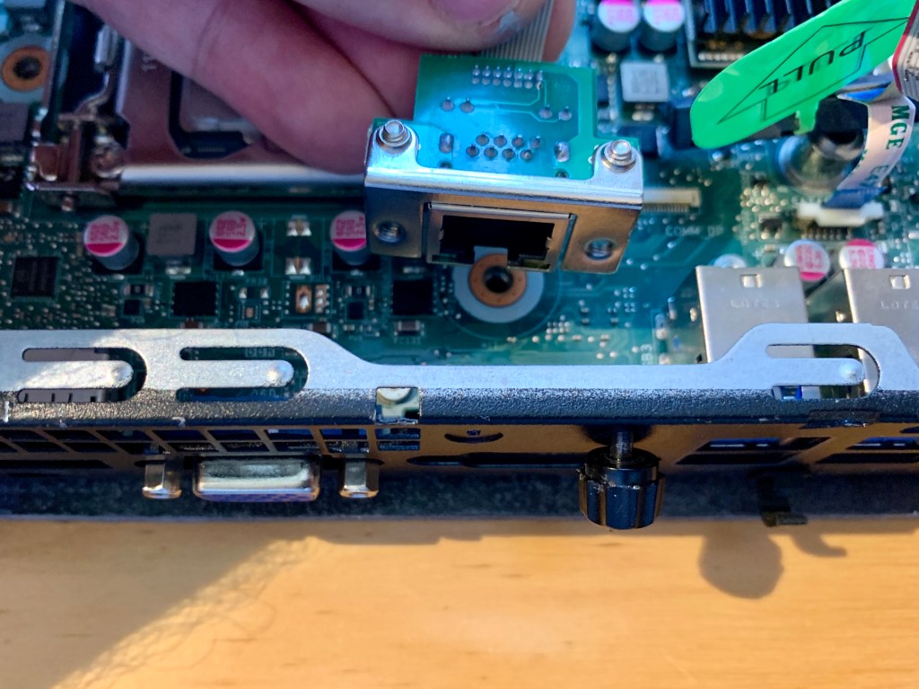
Correct orientation of the RJ45 port
Offer up to the RJ45 port to the opening left by the daughterboard. Check that the orientation matches the above photo, i.e. cable latch and LEDs should be towards the bottom of the machine. Loosely hold the RJ45 port in place with the M3 bolts and washers, but allow it to move for now.
Refitted heat sink shroud
Refit the modified heat sink shroud by clipping it back into place. Check that the RJ45 port is still free to move a little and is not being obstructed by the shroud.
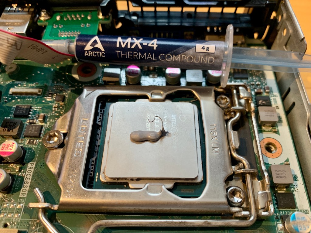
Reapply thermal paste
Apply some fresh thermal paste to the CPU, in preparation to receive the heat sink.
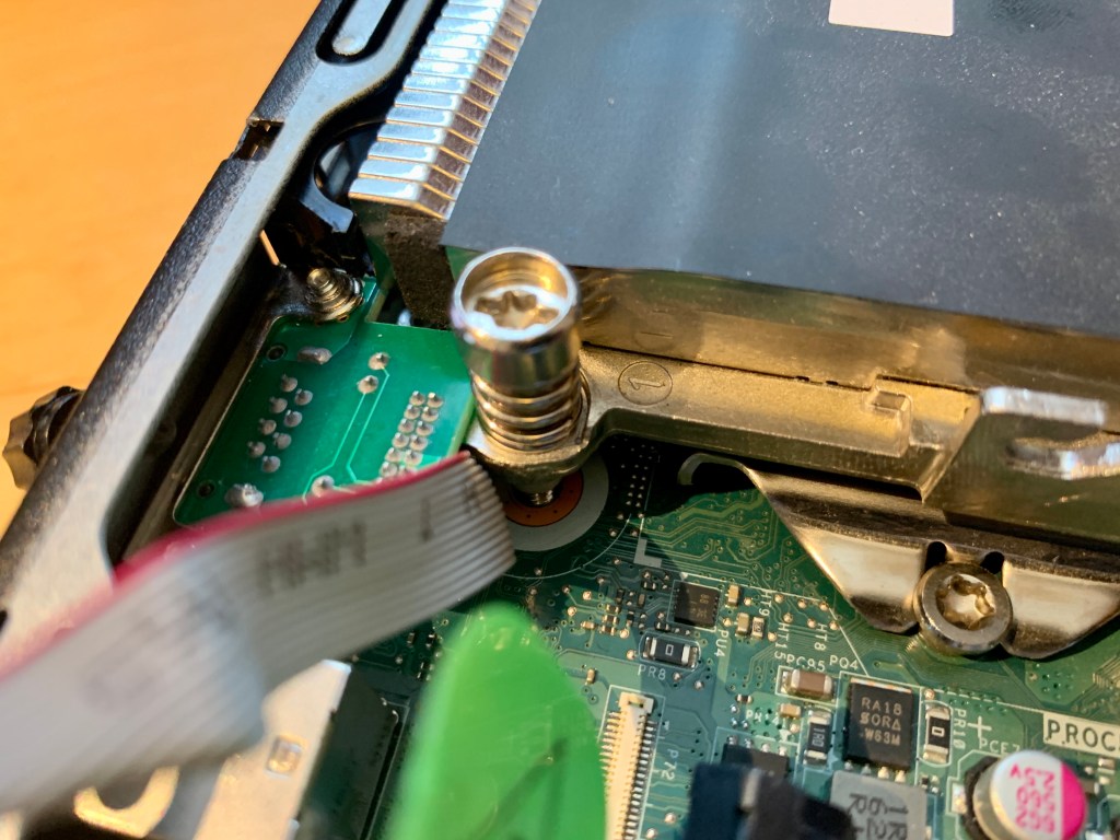
Refit the heat sink. This is the most fiddly stage of the process. You must lift the edge of the loosely-fitted RJ45 port to allow the heat sink to pass under it. Bend the cable out of the way, fairly sharply. When you tighten down the heat sink bolts, triple check that you have not pinched the cable, and that it hasn’t been pulled off the connector. Use a flat screwdriver to carefully push the cable back onto the connector if the heat sink tugs at it.
Refit by fan unit by sliding the black pegs into the grooves, and lowering the fan into place. It doesn’t click; it just rests on top of the memory.
Carefully tighten the M3 bolts on the rear of the case, taking care that the washers are aligned with the edges of the cut-out, and do not obstruct the USB ports.
With both components firmly fixed in place, route the cable around the edge of the case. Take special care not to dislodge the SATA cable, and ensure that the cable runs down the side of the CMOS battery and not over it, or it will get pinched by the drive cage.
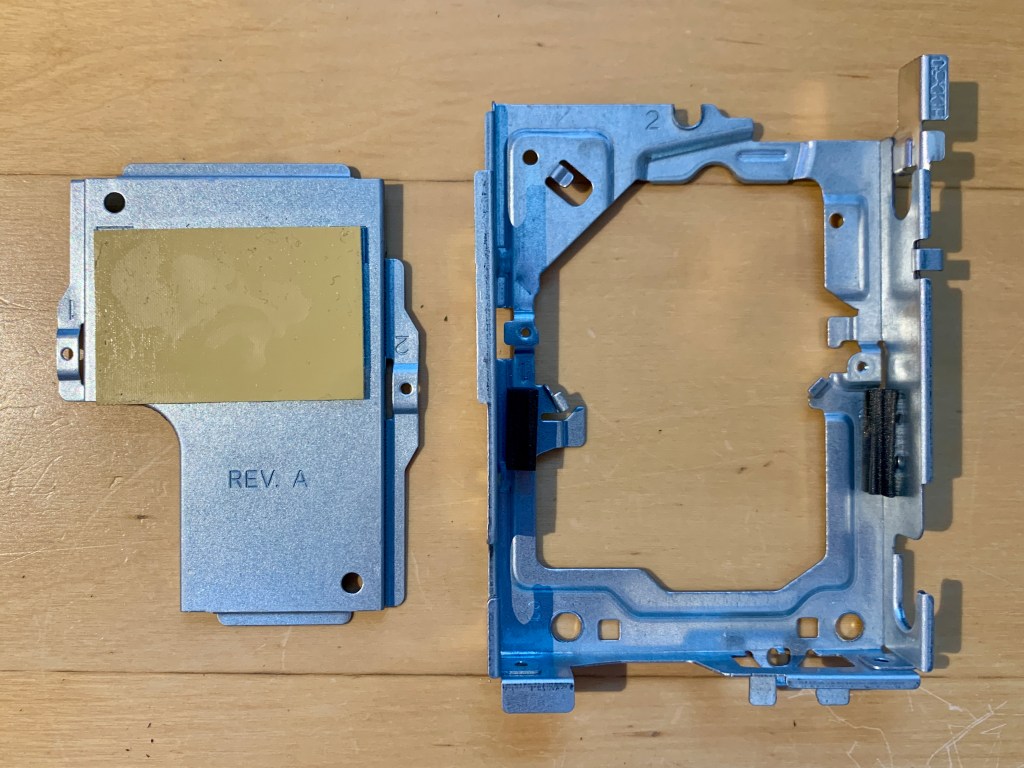
Disassembled drive cage
Take the drive cage, and remove two small screws to take out the piece stamped Rev. A. Discard this piece.
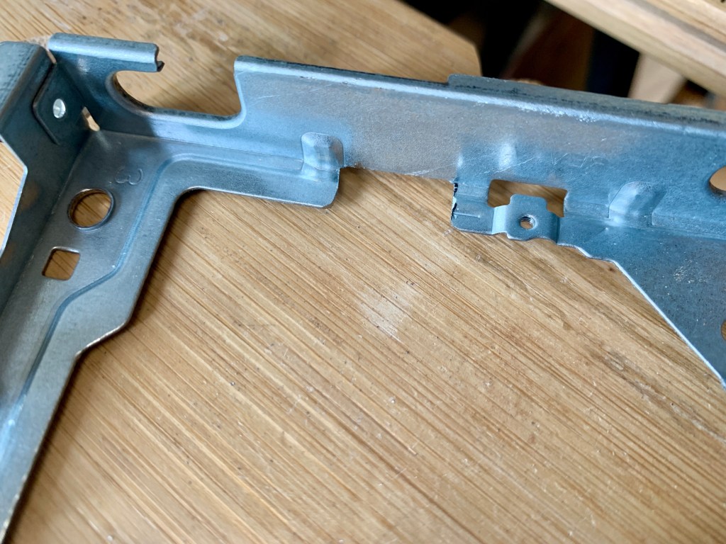
Drive cage with cut lines
If you try to refit the drive cage now, you will find that it fouls the connectors on the 2.5GbE card. Peel off and discard the chunk of foam on the left hand side.
Use a junior hacksaw (or Dremel) to cut along the two lines I have drawn on the cage above with black pen. Use pliers to bend this piece back and forth a couple of times until it snaps off at the folded edge. Use a file to remove any sharp corners and burrs, and be sure to remove all metal filings so they don’t get into the PC.
The modified drive cage
When your drive cage looks like the photo above, you can refit it with the three bolts. Check that the grey ribbon cable is not snagged or pinched by the cage. Remember to slide the case open sensor back into place on the front of the cage.
HP G2 Mini with modified drive cageedge
With the drive cage refitted and the ribbon cable comfortably in place, refit the SSD by sliding it into place and carefully refitting the SATA cable.
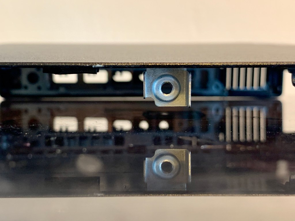
Finally, you will need to trim the retaining catch on the case lid, otherwise it will foul the RJ45 port.
Factory design of retaining nut
The retaining nut on the lid already has a corner cut out. Trim the whole nut in line with that cut-out using a hacksaw and file, taking care to remove all metal filings.
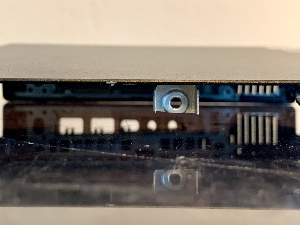
Modified retaining nut
With the edge trimmed off, the retaining nut will work just as well, but it will now fit without damaging the RJ45 port. Replace the lid.
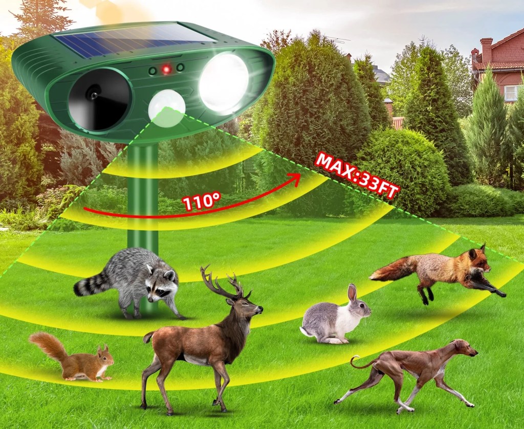
A house I walk past on the school run has recently installed an ultrasonic animal scarer – presumably to deter the urban foxes that are prevalent in the area. These devices are supposed to emit ultrasound that is too high for humans to hear, but makes a frightening or unpleasant noise for animals, who have much more sensitive hearing. They are triggered by motion, via an infrared sensor.
Product image of a typical ultrasonic animal scarer
I noticed that I was able to clearly hear this animal scarer – it appeared to me as an unpleasant squealing or fizzing sound. I can’t think of a better way to describe it other than “it sounds like a migraine”. My 8-year-old daughter was able to hear it much louder than I was, to the point that it was physically uncomfortable for her. We always have to run past the house with her ears covered!
This got me thinking. The range of human hearing is widely said to be from 20Hz at the low end, up to 20,000Hz (or 20kHz) at the high end. As we age, the upper limit of our hearing reduces with healthy adults typically able to hear up to around 15-17kHz. These characters vary widely between individuals, but generally:
In my late 30s, I can hear all of those tones except 17,400 Hz. However I can feel some sort of weird sensation in my ears, so presumably it’s about on the threshold for me. With that in mind, why am I able to hear the “ultrasonic” animal scarer so easily? Surely that should be well above 20kHz, where no human could possibly hear it.
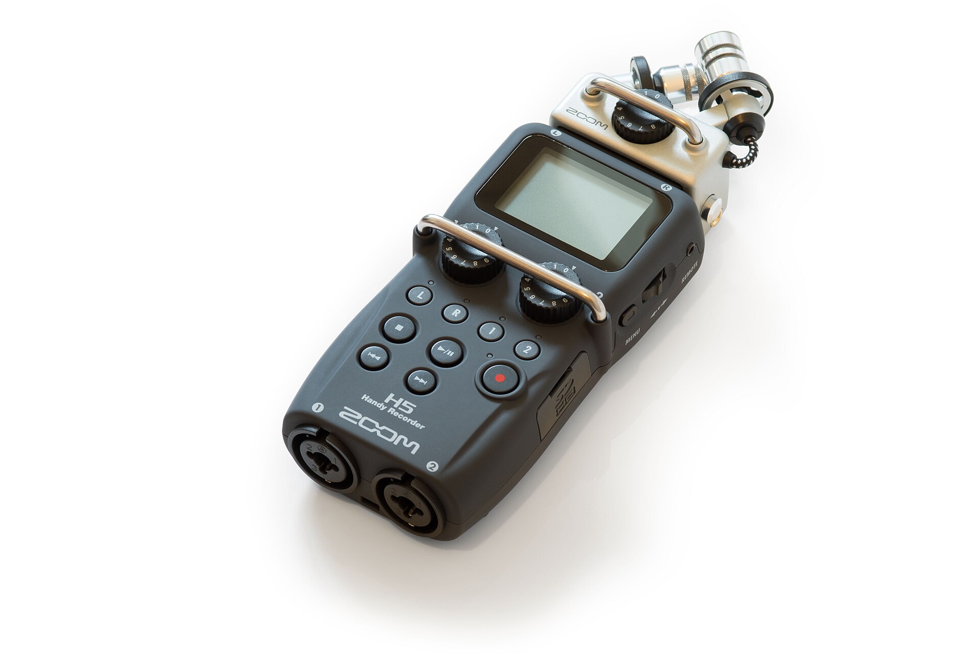
I don’t have any proper way of measuring ultrasound, but I do have a handheld Zoom H5 recorder. It is capable of recording uncompressed audio at a sample rate of up to 96kHz, so according to Nyquist’s law, it is theoretically capable of recording frequencies of up to 48kHz. I have no idea whether the microphones and circuitry are that sensitive, or even if frequencies above 20kHz are filtered out.
A Zoom H5 portable recorder
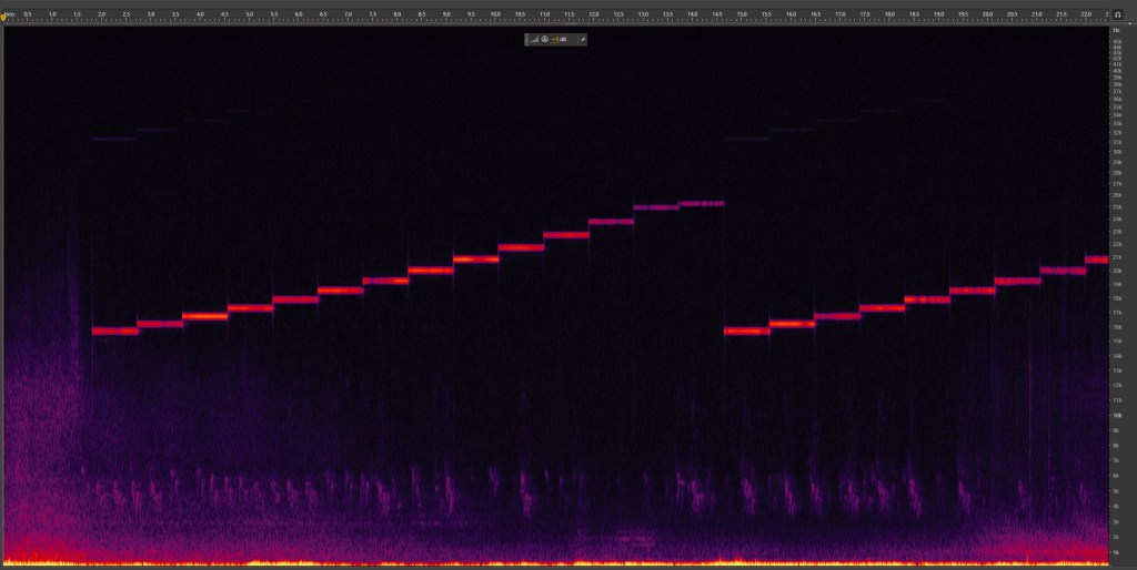
The next day, on the way to school, I took my recorder and captured the sound of the animal scarer. It was triggered by the motion of me walking past the house, and I was able to hear two bursts of ultrasound, a few seconds apart. Then I inspected the sound file in Adobe Audition, and used the spectral frequency display to make this plot. Time goes from left to right, and frequency goes up.
Spectral frequency display of the animal scarer
We can see from the plot that the Zoom H5 was easily able to record frequencies above 20kHz. We can also see that the ultrasonic animal scarer plays a scale of ascending notes, twice. This is why it appears as two bursts to me – I can apparently only hear the first few notes of the scale. You can even see that I stopped the recording because I thought the burst had finished.
If we look at the frequency scale on the graph, we can see that the lowest note of the scale is around 16kHz and the highest is around 21kHz. This is a pretty inconsiderate range, as virtually all children and young adults will be able to hear some or most of the sound. Even at the age of 38, I can hear the first three notes. And that’s before we even consider that the evidence is pretty mixed on whether they even work for keeping animals away at all.
I don’t really know what to do with this new-found information. Is it the done thing to knock on people’s doors and show them spectral frequency graphs? Like a religious preacher, but with science?
For those of us who run Kubernetes on-premise on physical hardware, it is entirely possible that not all your nodes have the same hardware. For memory and CPU cores, Kubernetes magically does the right thing and each node advertises how many cores and how much memory it has, and workloads are scheduled on a node that has sufficient resources.
For other hardware (commonly GPUs) or if you need to match specific CPU features, there is an excellent tool called Node Feature Discovery (we’ll call it NFD for short) which scans your node hardware and labels the Kubernetes nodes with various key/value pairs – some are boolean flags while others are quantities. You can see your labels with the following command. The output is long, so I have truncated it here.
$ kubectl get node kube04 -o jsonpath='{ .metadata.labels }' | jq
{
  # Examples of CPU features (e.g. instruction sets)
  "feature.node.kubernetes.io/cpu-cpuid.ADX": "true",
  "feature.node.kubernetes.io/cpu-cpuid.AESNI": "true",
  "feature.node.kubernetes.io/cpu-cpuid.AVX": "true",
  "feature.node.kubernetes.io/cpu-cpuid.AVX2": "true",

  # Example of other system values
  "feature.node.kubernetes.io/cpu-hardware_multithreading": "false",
  "feature.node.kubernetes.io/cpu-model.family": "6",
  "feature.node.kubernetes.io/cpu-model.id": "94",
  "feature.node.kubernetes.io/cpu-model.vendor_id": "Intel",
  "feature.node.kubernetes.io/kernel-version.full": "6.5.0-28-generic",
  "feature.node.kubernetes.io/kernel-version.major": "6",
  "feature.node.kubernetes.io/kernel-version.minor": "5",
  "feature.node.kubernetes.io/kernel-version.revision": "0",
  "feature.node.kubernetes.io/pci-0300_8086.present": "true",
  "feature.node.kubernetes.io/storage-nonrotationaldisk": "true",
  "feature.node.kubernetes.io/system-os_release.ID": "ubuntu",
  "feature.node.kubernetes.io/system-os_release.VERSION_ID": "22.04"
}
My specific use case is to inspect the network hardware and label nodes according to the speed of their network adapters. I have a physical cluster of 6 bare metal nodes and I’m halfway through upgrading them from gigabit Ethernet to 2.5G Ethernet. I would like the ability to pin specific bandwidth-hungry workloads to the nodes with the 2.5G networking.
NFD doesn’t include labels related to networking out of the box, but it does have access to a lot of extra information behind the scenes, and it provides several CRDs to enable you to access them.
NFD has a concept of Features, which is a piece of information that NFD has discovered about a node. The list of all currently available features is available in the docs, and it shows that there is a feature called network.device which includes the speed of each network interface, in Mbps, as a string.
The other piece of the puzzle is to “match” this feature by creating a NodeFeatureRule, which allows you to set conditions based on Features and use them to generate labels to be applied to the node. Here is a simple NodeFeatureRule that I have written to add labels for the network speed, based on which network interfaces are up.
This is an article about the ancient traditions of the Christian Church, and the modern principles of developing software. Probably not much of an intersection there!
Seasons
For those who don’t know, most churches have a concept of liturgical seasons and colours. These vary a bit between denominations (i.e. Anglican, Catholic, Protestant, Episcopal, Lutheran, etc) and countries, so for this article I’m specifically talking about the Church of England, which is a member of the Anglican Church. There is a lot of jargon involved so I’ll try and keep to plain English wherever I can – that includes church jargon and software jargon!
Some seasons, everyone will have heard of (like Advent, Christmas and Lent) but there are some other seasons that you might only know about if you go to church (like Pentecost and Trinity). Some of these seasons are related to Christmas – which has a fixed date every year, and some are related to Easter – which moves around each year according to the cycles of the moon.
On top of the irregular seasons, there is a calendar of Holy Days which includes the big days that everyone knows (Christmas and Easter) but also many days throughout the year dedicated to saints, martyrs and Biblical events. There is a priority system to work out what happens if one of the movable days like Easter happens to land on one of the non-movable days. Sometimes they share, and the day therefore marks both dedications. Sometimes the more important dedication cancels the less important dedication. If a dedication is cancelled, sometimes it gets shunted to a different day. Other times it just gets skipped for that year.
Colours
Each season has its own colour which is typically reflected in the altar hangings (tablecloths), the garments worn by the priest, other decorations around the church building, and maybe even the flowers that are on display.
Example of liturgical colours in garments
Some, but not all, of these Holy Days have their own colour which overrides the colour of the season.
Rules
All of these rules mean it is rather complicated to work out what this year’s seasons are, what dedications fall on which days, and what the colour is. Fortunately, the Church of England publishes an annual book called the Lectionary, which is basically a calendar that contains all of that year’s information about seasons, Holy Days, colours, readings, etc. This is usually good enough for typical church business like planning services and remembering when to change the altar hangings.
The Church of England Lectionary
Algorithm
It’s not good enough for me, though. I want a way of automatically working out the dates, the seasons, and the colours. This means I have to reimplement the same algorithm used to work all this stuff out, and then seed the algorithm with a list of Holy Days.
I looked around for existing open-source projects that can calculate liturgical dates and colours. There were a few, but they were mostly focused on the Roman Catholic Church, and none of them were written in languages I knew well.
Then I found a Perl module called DateTime::Calendar::Liturgical::Christian which is aimed at the US Episcopal Church, which seems to have a fair bit of commonality with the Anglican church. I know a bit of Perl, so I ported this module to Python (the main language I use now), tweaked the algorithm to reflect the Church of England’s seasons, and replaced the Episcopal Church’s Calendar of the Church Year with the Church of England’s Calendar of Saints, along with its revised priority system.
The end result is a Python library that I have called Liturgical Colour, and which is published on PyPI. Here’s sample output when run for 31st March 2024 – Easter Day:
name : Easter
url : https://en.wikipedia.org/wiki/Easter
prec : 9
type : Principal Feast
type_url : https://en.wikipedia.org/wiki/Principal_Feast
season : Easter
season_url : https://en.wikipedia.org/wiki/Eastertide
weekno : 1
week : Easter 1
date : 2024-03-31
colour : white
colourcode : #ffffff
The output is basic, but includes all the key information – including the name of the colour and the HTML colour code, which leads neatly onto the next section.
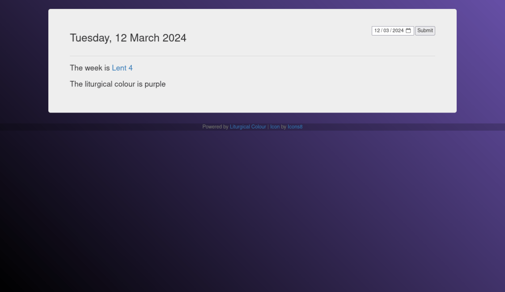
App
Now we have a library that can calculate all the required information for any date, we just need a way of displaying the information. I’m no frontend developer, but I managed to throw together a simple Python app based on Flask which uses the Liturgical Colour library and renders a simple display for the user.
Here are some screenshots of example output from different dates. There are also two days per year when the app will display rose pink!
I’ve been using Facebook since 2006, back when it still required a college or university email address to sign up. These days, I use it for two main purposes:
To keep up with friends and family
To participate in groups related to my interests
My use of Facebook groups to discuss and read about my interests has more-or-less completely replaced my use of forums and mailing lists for this purpose.
Recently, I’ve noticed an increasing number of posts in my feed that are not from groups or pages I follow and it feels like the whole thing is inundated with sponsored ads.
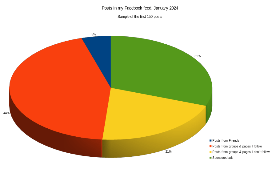
So I decided to do a little survey, and I scrolled through the first 150 items in my feed, categorising them into the following:
Posts from Friends – exactly what it says on the tin.
Posts from groups & pages I follow – for example, groups like Woodworking UK that I have joined
Posts from groups & pages I don’t follow – groups and pages that Facebook thinks I might be interested in, even though I haven’t joined
Sponsored ads – mostly picture and video ads which link to external sites like Amazon
This is not a discussion on how Facebook decides what to show me, and how “the algorithm” uses my personal data – merely the composition of my feed.
Posts from Friends
7
5%
Posts from groups & pages I follow
66
44%
Posts from groups & pages I don’t follow
31
21%
Sponsored ads
46
31%
It seems my gut feeling was correct! About a fifth of my feed consists of items from pages and groups I don’t follow, and a third is sponsored ads. In total, a little over half my feed is content that I didn’t ask for!
I saw ads from a variety of sectors – technology, food & drink, holidays, clothing, entertainment, and I saw some of the ads several times.
The content from groups I don’t follow is irritating to me. For example, I like classic Jaguars (the car, not the big cat) and so I’ve joined a couple of groups dedicated to Jaguars. “The algorithm” has picked up that I like cars, and a lot of the content it shows me is from groups dedicated to other cars (such as BMWs), or other geographic areas (such as the Pittsburgh Classic Car Meet).
I noticed that some of the posts from friends were several days old, so I don’t know why they are only now appearing in my feed.
I don’t have data to back this up, but I believe Facebook is prioritising content from groups over content from friends, and making a big effort to users into as many groups as possible and to follow as many pages as possible, not to mention serving as many ads as possible. It feels like its usefulness to me is declining.
It’s a question I’ve heard asked quite a few times: why don’t EVs have solar panels on the roof? Then they wouldn’t need to be charged with a charger, would have infinite range, and would be using only green electricity!
It’s a fair question. To answer it, let’s have a look at some numbers.
How much energy do we actually get from the sun? Well, solar irradiance at the surface of the earth, the amount of sunlight energy falling on each square metre of Earth’s surface, is approximately 1100W/m². But this is an average figure across the whole globe. It is more at the equator and less at the poles. Here at my location in the UK at 51.5° North, my weather station has measured peak solar irradiance of ~1000W/m² at the height of summer. This limits the maximum energy we can ever get from the sun, regardless of the type of solar panels used.
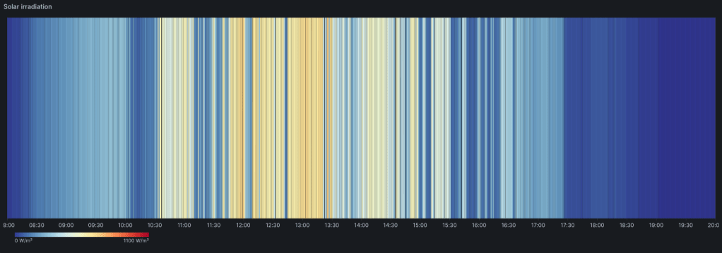
This graph shows the solar irradiance at my weather station over the daylight hours (08:00 – 20:00) of a typical sunny September day. The peak solar irradiance was more like 700W/m² with an average much below that. Note the gaps in the yellow/orange area, where clouds pass over.
Solar irradiance over 12 hours, September, UK
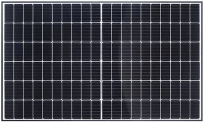
Let’s be generous, and take 700W/m² as our figure of solar irradiance. We must also account for the efficiency of solar panels. The conversion efficiency of commodity solar panels is only about 25%, which further reduces the amount of useful electricity we can extract down to 175W/m².
How large actually is a car roof? I’ve just been outside to measure the useful roof space of a typical family hatchback (a Hyundai i30) and it measured 1.0×1.7 m, for a total area of 1.7m². A larger family car (a Ford Mondeo) would be able to offer 1.1×1.9 m for a total of 2.09m² of useful roof area if the roof rails weren’t fitted.
2015 Ford Mondeo
The Mondeo is more comparable in size to a Tesla Model 3, so let’s run with those dimensions. Multiplying the available roof area for solar panels (2.09m²) with the average useful solar irradiance in the UK (175W) yields a total electrical power of 366W or 0.366kW from the roof of a large family car.
To put this into perspective, a typical home EV charger operates at 7kW – more than 19 times more power (and therefore 19 times faster) than on-roof solar charging. Standard chargers found in public locations are typically 22kW and rapid chargers are 43kW, which is 60 or 117 times more power than solar charging respectively. Which? has a good overview of charger types.
Staying with the Tesla Model 3, the base model has a battery pack rated for 50kWh, which is fairly typical for today’s EVs. With solar charging alone, it would take 137 hours (almost 6 days) to fully charge. But solar panels only work in daylight hours, so in summer it would take more like 12 days!
The available power is obviously reduced even further in the winter months, on cloudy days or if you park in a multi-storey car park or under a tree.
So I guess this is our answer – it’s just too underpowered and too slow to be practical.
But why couldn’t EVs come with solar panels on the roof for emergency backup? Just enough charging capability to make sure you don’t get stranded? Or to add a few miles to the range?
Well, they could. But cars are manufactured with slim profit margins and solar panels are an expensive component to include for such little benefit. It just doesn’t make business sense.
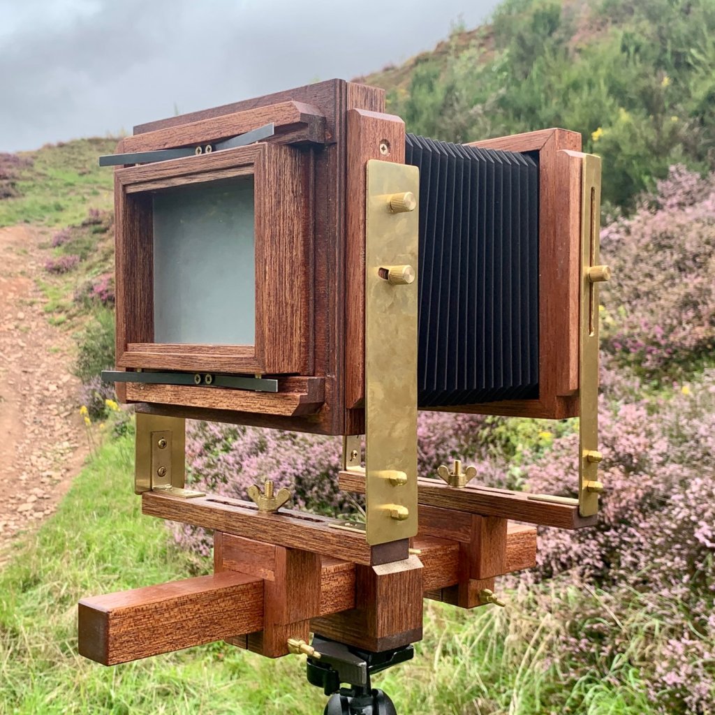
I’ve wanted to build a wooden large format camera for years, but I made myself wait until my skills were up to scratch. I reasoned that a wooden camera isn’t really too much more difficult than a sort of trinket box / picture frame hybrid, so I decided to take the plunge.
I looked at various plans for cameras that are available online, but eventually decided to follow Jon Grepstad‘s freely available plans for a monorail camera – partly because his instructions were complete and contained diagrams, and partly because his measurements were in metric. Can’t be doing with sixty-fourths of an inch!
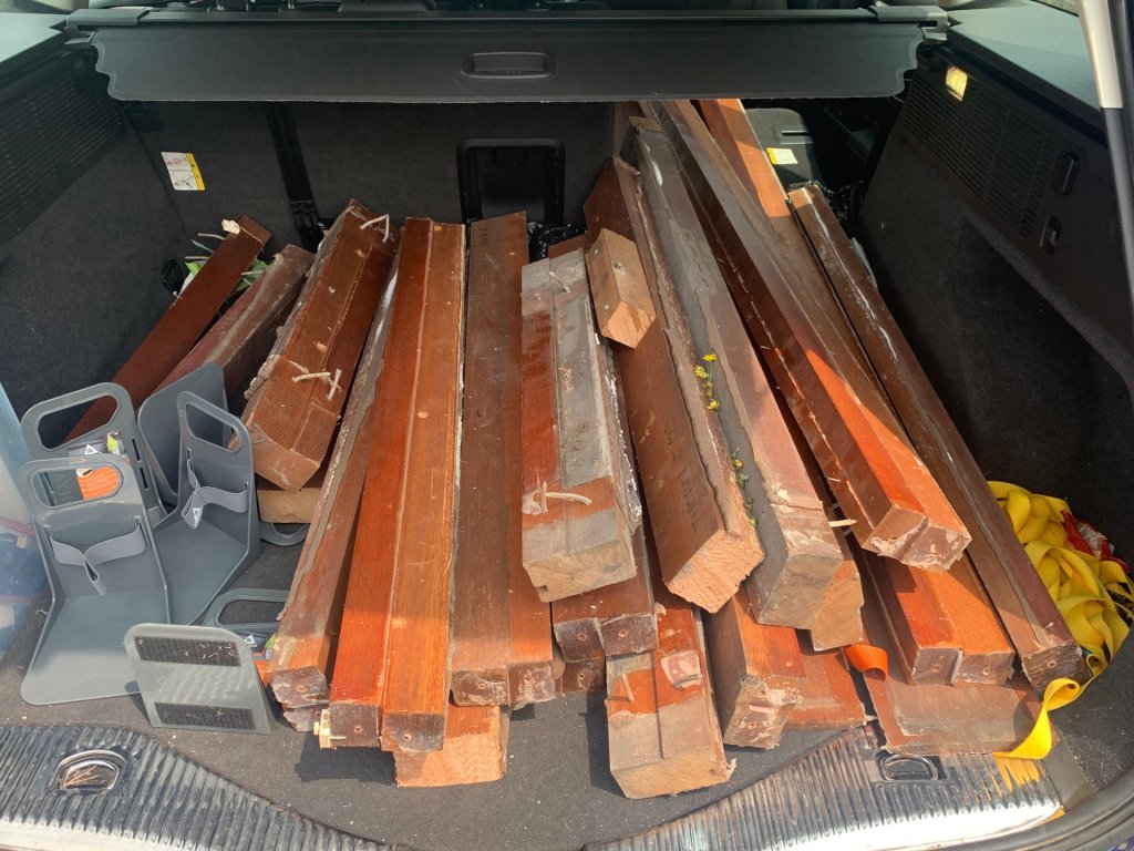
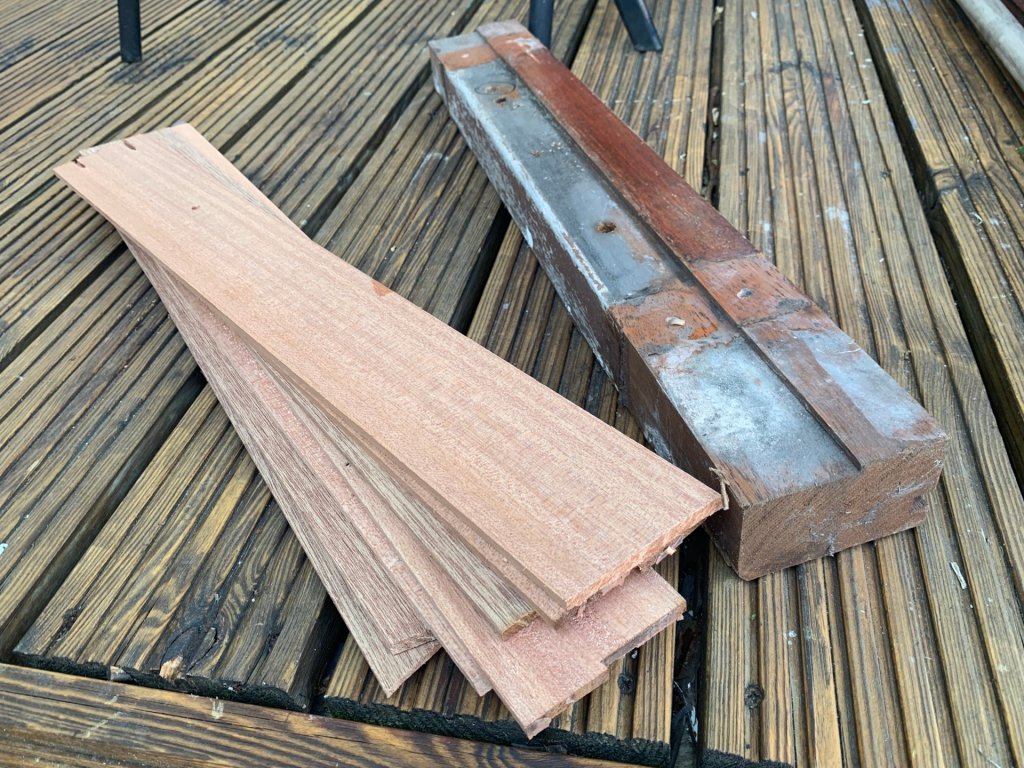
My decision to get started was cemented when I found some wooden window frames being ripped out. I saved them from the skip, and they turned out to be meranti, sometimes also known as Philippine mahogany. It’s a hardwood commonly used for window frames, because of its resistance to warping when it gets wet. My camera won’t need to withstand bad weather, but the reddish hue of meranti is very pleasant.
Salvaged meranti window frames
Preparation
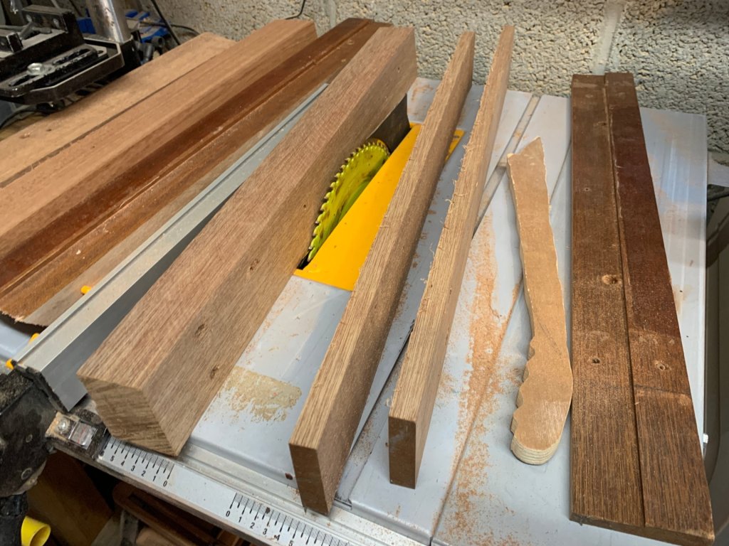
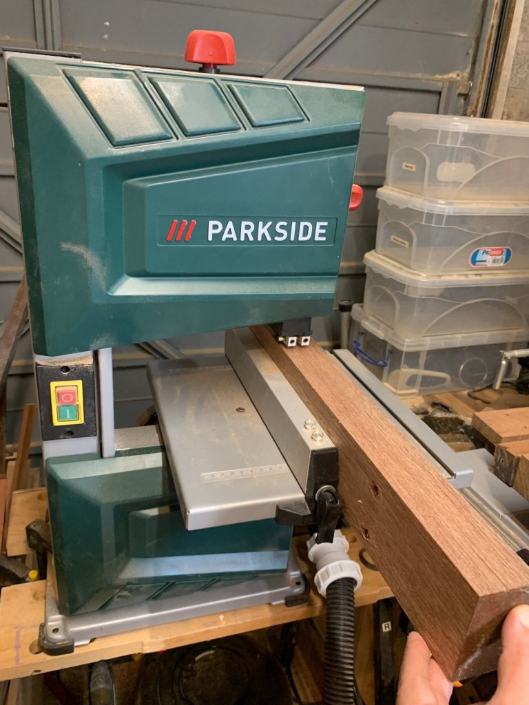
The meranti needed a bit of a clean-up – first scraping off remnants of glue and sealant, and secondly checking carefully for screws and nails, and removing them. The camera plans call for thin boards of meranti ranging between 6mm and 15mm rather than thick chunks, so I ripped these pieces on my table saw to reduce them down to an 80mm width that my band saw can take, then used the bandsaw to resaw them into boards that were slightly thicker than required. Finally I passed them through the thicknesser to reduce them down the precise dimension and leave a nice, planed finish. The old varnish and effect of weathering had only gone into the wood a couple of millimetres so I was left with beautiful fresh timber and no indication that it had been window frames for decades.
Ripping on the table sawResawing on the bandsawThe meranti boards ready to use
Construction
I didn’t actually remember to take many pictures of the construction process, but there was a theme with the woodwork side of the project: further rip the planed boards into narrower strips, and then glue them back together in various L-shaped profiles as specified in the plans. Then almost all of the camera parts are cut from these long L-shaped profiles with a mitre saw, working around the occasional nail hole, and assembled in the same way as a picture frame with ordinary wood glue. Band clamps came in very handy here.
Front and rear frames complete, balanced on sliders and monorail
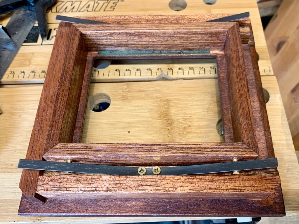
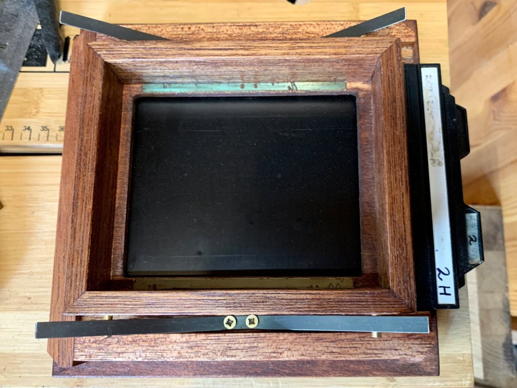
I used plywood for a couple of parts, such as the lens board, and the main body of the spring back film holder. The spring back holder is perhaps the most complex part of the build, as the ground glass focusing screen is held to the back of the camera by leaf springs, and when it’s time to take a photo you slide the film holder underneath the ground glass, which springs up, clamping the film holder in place and ensuring that the film is in the same plane that the ground glass was in during focusing.
Spring backSpring back with film holderSpring back with film holder
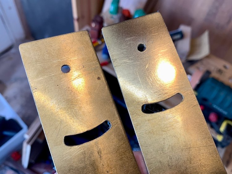
One aspect of this project that was totally new to me was metalwork. I’ve never worked with brass before, but I was pleasantly surprised how easy it was to cut 1-2mm brass sheets on the bandsaw, drill on a pillar drill and work with a file by hand. The parts I needed to make were all simple, but it took quite a lot of effort to sand and polish out the tool marks.
Rear standards with curved slot
Jon Grepstad’s plans described a rotating back system, but I decided to omit this as I rarely shoot in portrait orientation, and it seemed like an opportunity to save a little weight and complexity.
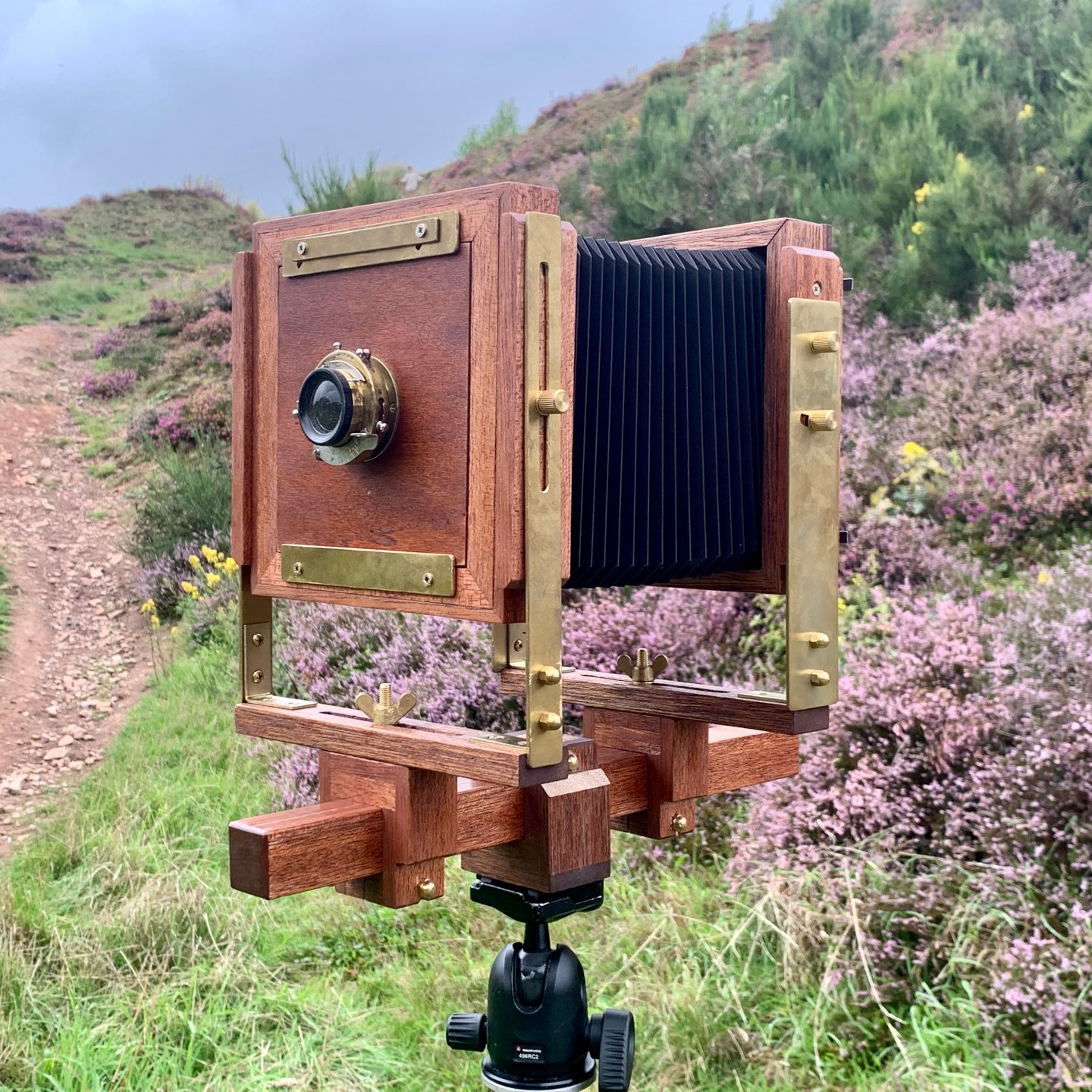
I completed the build by adding a bellows and ground glass I ordered from a photographic supplier, and a lens I salvaged from a broken camera. The bellows is conveniently the same dimension as a Toyo 45G. The ground glass is the traditional, non-Fresnel variety and the image is quite dim, but I don’t mind that. The lens is a Bausch & Lomb Rapid Rectilinear in a Kodak shutter, dated 1897. The focal length isn’t given but the maximum aperture is US 4 (Uniform System, not United States), equivalent to f/8.
To really bring out the mahogany colour and deepen the pinkish-red shade of the meranti, I finished with several coats of mahogany-tinted Danish oil. This also gives the wood a pleasant sheen rather than a high gloss finish.
Tools
I wanted to make a quick note about the tools I used. There’s a lot of discussion on the various woodwork groups online about the “best” tools and how cheap tools aren’t even worth bothering with.
I’m using budget tools exclusively, and while the build quality and precision aren’t always great compared to expensive brands, they have been sufficient for my modest needs as a hobbyist. With careful setting up and use of tools, I’ve managed to achieve sufficient precision.
Titan TTB579PLN planer/thicknesser
Titan TTB763TAS table saw with Saxton blade
LIDL Parkside PBS 350 band saw with Tuffsaws blades for wood and metal
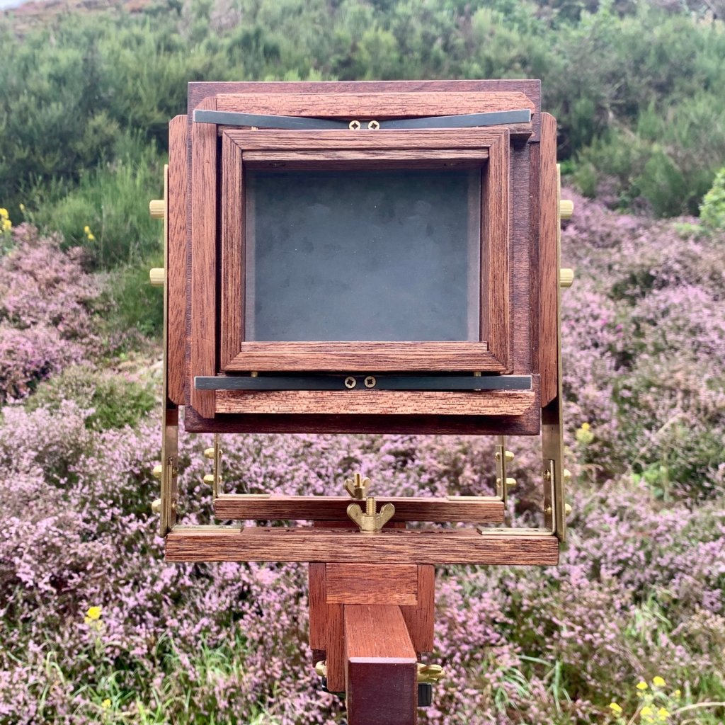
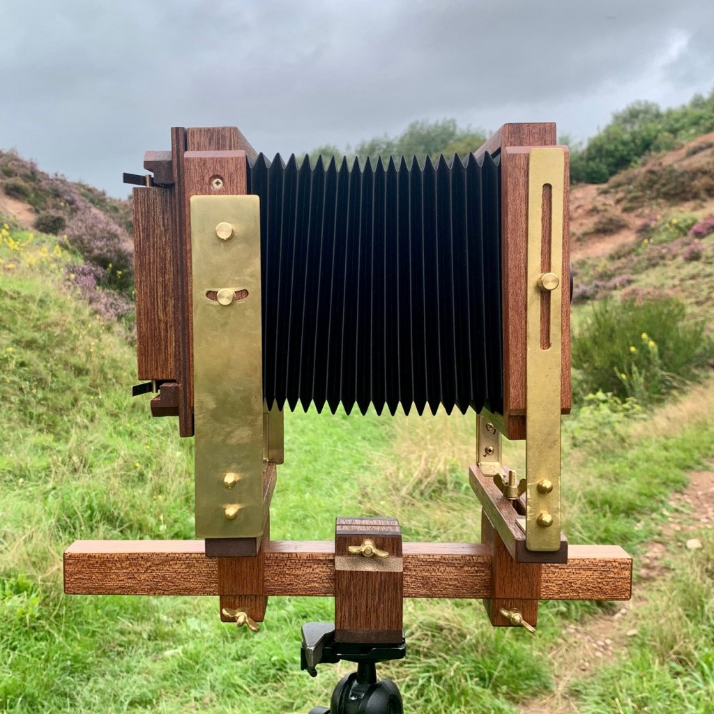
Front viewFront viewRear viewFront quarter viewRear quarter viewSide view
Movements
A key part of the specification of any large format camera is its movements. The length of the monorail is 380mm so this allows for generous extension of the bellows at typical focal lengths.
Front
Rear
Rise/Fall
+55mm, -35mm
0mm
Shift
±50mm
±50mm
Tilt
Limited only by bellows
±20°
Swing
Limited only by bellows
Limited only by bellows
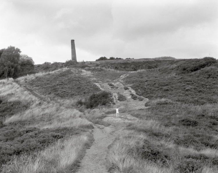
Testing
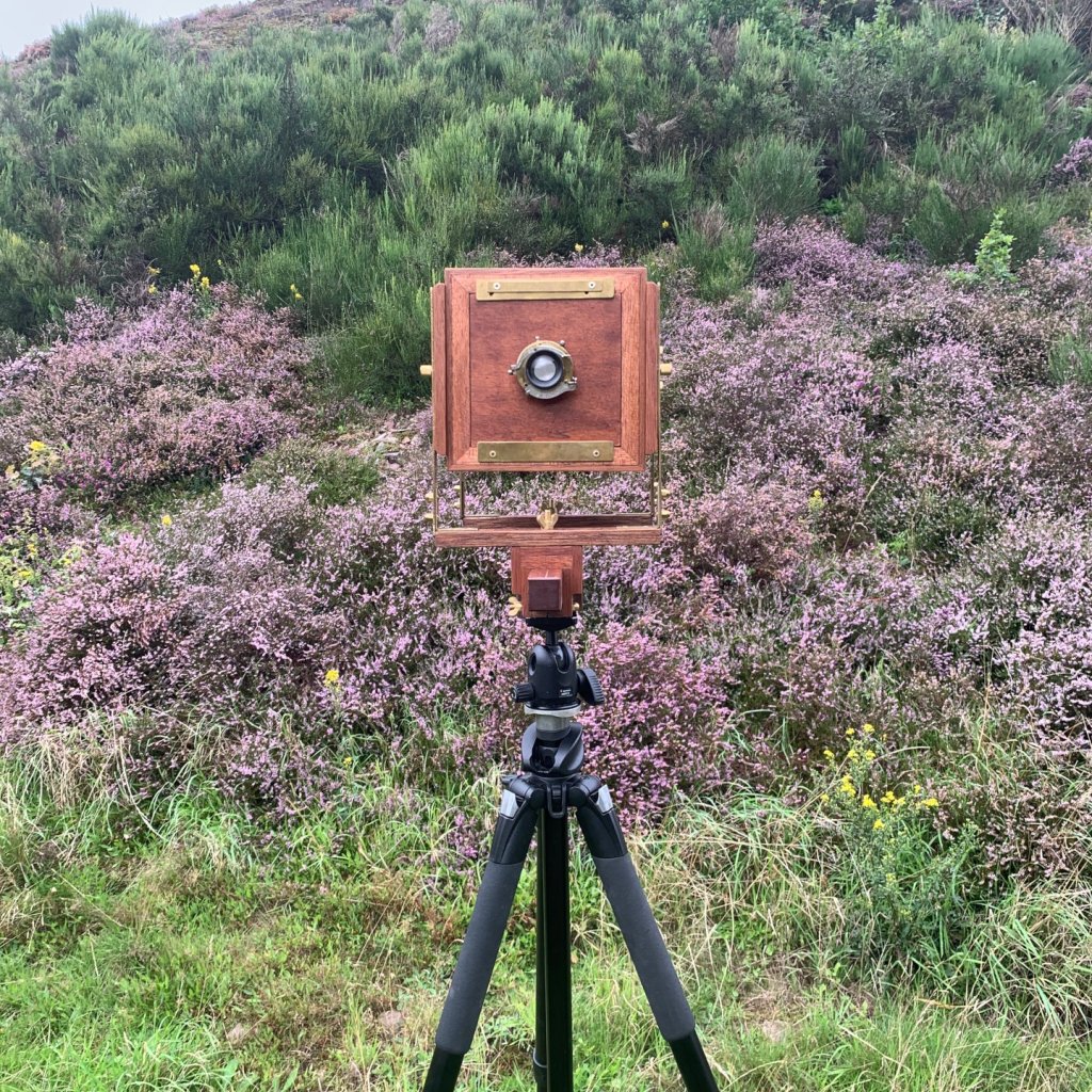
Here’s the first test shot taken with this camera, also at Trooper’s Hill.
Trooper’s Hill, Bristol
I’m really happy with the results. For a lens that is 126 years old, it has good, even coverage and decent sharpness at f/16, two stops down from wide open. There is no evidence of light leaks.
I slightly missed critical focus, and I think that’s largely because I used wood for the monorail instead of the recommended aluminium tube. The varnish-on-varnish sliding made it quite hard to make tiny adjustments accurately. Hopefully waxing the monorail will help with a smoother action..
I also found that the leaf springs I chose are slightly too strong and clamp down on the film holder slightly too hard. You have to be quite forceful when inserting the film holder, and it is quite easy to accidentally knock the alignment of the camera. Hopefully I’ll be able to bend the springs a bit so they’re not quite as aggressive.
Finally the last thing I noticed while using the camera is that it can be quite tricky to get it aligned when setting up. None of the adjustments have a centre “click” detent, so you have to take your time aligning and adjusting when composing an image. This isn’t a fast camera to use!
Overall, I am very pleased with my first camera build. It has turned out well, and I have made a usable camera that I cam proud of, and learned some new skills along the way. I’m also very grateful to Jon Grepstad for publishing his plans.
I recently received an Ecowitt WS2910 weather station for Fathers’ day. I’ve always wanted a weather station so I was very excited. This isn’t supposed to be a review of the product, but I think it would be helpful to go over the basics before we dive into the meat of this blog post (the integration with Prometheus).
Ecowitt WS2910 weather station
The outdoor portion of this weather station (model number WS69 if you buy it separately) measures wind speed, wind direction, temperature, humidity, rainfall and solar irradiation. It takes AA batteries which are supposed to last for 2-3 years as it gets the bulk of its power from the solar panel during daylight hours. There are several different Ecowitt weather stations which include the same sensor array.
The sensor array communicates with the indoor base unit periodically, via UHF radio. My model uses 868MHz but judging by the box, there are at least 4 different frequencies available for different parts of the world. The base unit doesn’t need pairing with the outdoor part like a Bluetooth connection – it just waits for the next radio signal to come in and starts displaying data.
The base station is simple but effective. It shows almost all the information you want on the main screen (not a touch screen), and there are several touch-sensitive buttons that let you change view or look at old data. This is a bit fiddly, so I’m just using it as a “current status” dashboard and not touching the buttons. It’s also not a true colour screen, but a backlit LCD which seems to have coloured filters over the backlight to illuminate each section.
Ecowitt sell several different WiFi-enabled base stations and the main differentiator seems to be the size and quality of the screen. All of the models that have WiFi appear to behave the same way when it comes to data logging and integration with various online weather services. At the time of writing, everything from here onwards in this blog post should apply at least to the following models (and I’d love to hear from you if you find this works or doesn’t work for your model):
Ecowitt WS2910 with colour LCD display (this one)
Ecowitt WS2320 with mono LCD display
Ecowitt HP2551 with colour TFT display
Ecowitt HP3500B with colour TFT display
Ecowitt GW1101 headless weather station, no display
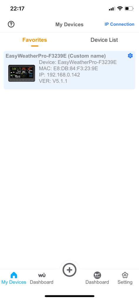
What I’m really interested in are the different options for integrations. There’s a smartphone app called WSView Plus (for iOS and Android) which pairs with the base station via local WiFi and allows you to configure your real WiFi network name and passphrase. It also allows you to set up integrations with various weather services, including the manufacturer’s own service Ecowitt Weather, Weather Underground, Weathercloud, and the Met Office.
WSView Plus device screenWSView Plus Ecowitt dashboardWDView Plus custom integration
The Ecowitt Weather service requires authentication to see the weather data, so it’s no use for sharing with other people. Weather Underground has a nice dashboard which is publicly available, so I registered as station IBRIST302.
There is also the option for a “custom” integration to send weather data to a custom endpoint. There are no details in the manual about the format of the protocol but from reading it seems that the Ecowitt weather station sends the data as an HTTP POST request with form encoded data.
I had a look around to see if anyone else had already written a tool that could receive data from the Ecowitt for local processing:
Almost all of the existing solutions very sensibly use InfluxDB, and that’s probably what you should use if you don’t have any existing infrastructure. However, I don’t want to run a new service unless I have to – and I already have a Prometheus instance that I want to import the weather data into. So I set about writing an exporter that could receive the HTTP POST requests from the weather station, transform the data where necessary, and present it where it can be scraped by Prometheus.
In the end I took parts of pa3hcm/ecowither and parts of bentasker/Ecowitt_to_InfluxDB, removed the InfluxDB bits and added the official Prometheus Python client to create an exporter. I included code to select output in Metric/SI or Imperial, and to toggle this independently for each instrument, to cope with the slightly odd “hybrid British units”, because we like most things in metric, except for wind speed, which we prefer in mph.
I did run into a bug where a malformed HTTP header being sent by the Ecowitt on firmware version v5.1.1 was causing bad behaviour in Flask. At the time of writing there is a PR in the pipeline to fix this, but I worked around the problem by fronting my Flask server with an NGINX reverse proxy – no special config required. NGINX seems to magically fix the broken header in flight.
But wait! That’s not all. If you simply run ecowitt-exporter, all it does is host an HTTP endpoint and waits for Prometheus to scrape it, which you will have to configure manually.
But as I’m running Kubernetes, I’m also running the Prometheus Operator which supports automatically configuring Prometheus to scrape targets based on the ServiceMonitorcustom resource. I created an ecowitt-exporter Helm chart which installs ecowitt-exporter and configures a ServiceMonitor resource to enable scraping. It can optionally also configure an Ingress (which at the moment is required, to work around the header bug described above).
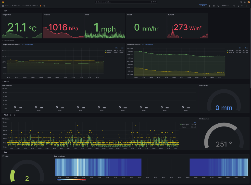
The last piece of the puzzle is a Grafana dashboard to visualise this data. I’ve tried to recreate the basic information shown on the weather station base unit, but with history. The top row is a “conditions right now” view, while all the other rows show 24 hours history (customisable).
Ecowitt dashboard for Grafana
At the time of writing, this dashboard is still evolving so I haven’t published it on Grafana’s list of community dashboards, but you can grab it from my git repo. It should “just work” if you are using the ecowitt-exporter for Prometheus. If you are using Grafana to visualise data from InfluxDB, this dashboard will need minor modification as the data sources will probably have different names.
All of these components are open source, so improvements, bug fixes, and new features are welcome.